Excel Tip – Swap Excel Columns Around
That was a quick month!
Swapping columns around is something that we do all the time in Excel. But it’s the way that we do it. What I usually see is people inserting a blank column, moving the data to that new column, then deleting the old column. That’s a lot of work!
- This is a feature that will make a difference to you every day in Excel.
You can view the video or follow the step-by-step shown below.
You’ll love this, so enjoy and remember: Keep it Simple!
Today, we’re going to see how we can swap 2 columns around in Excel, using a combination, of the keyboard and the mouse.
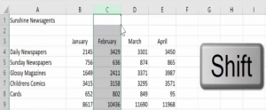
To demonstrate, I’m going to swap the February and March columns around.
Step 1 – Select the Column to be Moved
- Select the entire February column by clicking directly onto the C column heading.
- Then move the mouse to the right side of the highlight, until the cursor changes to a white arrow.

NOTE: This selection needs to be done on the sheet area, not on the column heading.
NOTE: You will also see 4 black arrows at the tip of the cursor, ignore these, it’s the main cursor you need to be looking at, and it should be a white arrow.
Step 2 – Engage the Mouse and Keyboard Together
- Once the cursor looks like a white arrow, click and hold down the click.
- Then hold down the SHIFT key on the keyboard.
- Drag to the right of the D – or March – column.
- At this stage you’ll notice that a green ‘T Bar‘ has appeared.

- That is exactly what you want to see, so you know you are doing it correctly!
- Once that ‘T Bar’ is positioned where you want the column to move to – release the click – then release the SHIFT key.
- February and March have now swapped places.

Isn’t that just wonderful?
Sigh…it really is the simple things in life that make us happy!
I’ll go through it again, and swap them back around – STAY AWAY from that Undo button – practice is good!
(Although I do love you, Undo button, so please don’t take offence…)
Step 3 – Select the Column to be Moved
- Select the entire February column by clicking directly onto the D column heading.
- Then move the mouse to the left side of the highlight this time, until the cursor changes to a white arrow.

Step 4 – Engage the Mouse and Keyboard Together
- Now you hold down the SHIFT key on the keyboard.

- And this time, we’re dragging to the left of the C – or March – column.
- Remember, if you see that green ‘T Bar‘ then you know you are doing it correctly!

- When the green ‘T Bar’ is correctly positioned, release the click, then release the SHIFT key.
Easy!
Thank you and I’ll be back with another useful tip next month!

OMG, so simple! I love it!
I’ve been doing this the LONGEST way for such a long time! Thanks, delighted with this tip.
Brilliant! I’ve been doing this the ‘long’ way for years
So simple now that I know it. Thanks!!!!
Very simple very good